Litho
A Python library for thermomechanical models of the Andean lithosphere. Its redesign around array operations made each model run 30 times faster.
- Lead developer, as research assistant to Dr. Andrés Tassara
- 2018–2022
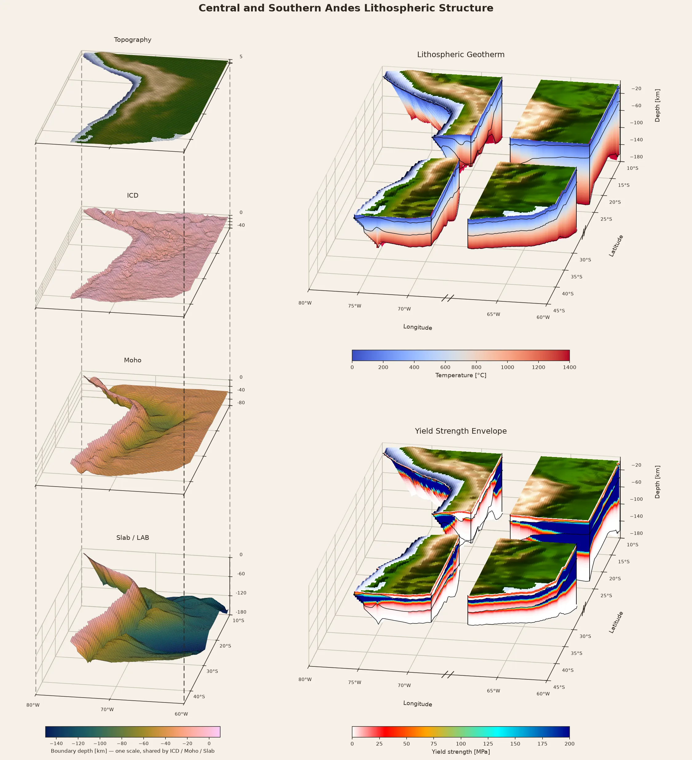
Litho models the temperature and mechanical strength of the lithosphere beneath the Andes, from the trench to the foreland, using the 3D geometry of its main boundaries. It was developed over four years in Dr. Andrés Tassara’s research group (Universidad de Concepción), where I was its lead developer: I wrote most of the code, including all of its core logic, and led its move to object-oriented design, purpose-built data structures and array operations. The research it supported was published in Earth-Science Reviews (Giambiagi et al., 2022) and presented at the EGU General Assembly (Tassara et al., 2020), with me as a co-author.
Physics first
The steady-state heat equation was derived analytically for three increasingly detailed versions of the crust, up to layers with their own heat production and their own thermal conductivity, checking the algebra with SymPy. SymPy also produced the inverse forms: the value of each thermal parameter that reproduces an observed surface heat flow, which became a tool of the library in its own right.
From loops to array algebra
Once moved from MATLAB to Python and extended with a mechanical module, the model still ran on nested loops and took about 90 seconds per run. Fitting it to observations took days. The redesign made every calculation run as 3D NumPy array operations over the whole study area.
- 30× faster: from about 90 s to 3 s per run, which made systematic parameter searches practical.
- Coordinate-aware arrays: a custom
ndarraysubclass carries coordinates with every result, so collapsing depth to compute surface heat flow always lines up. - No loops, even for the hard parts: detecting elastic layers and fusing their boundaries across the crust and mantle uses binary masks and array algebra.
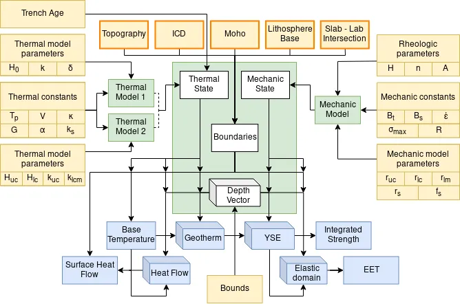
How the library fits together. Geometry (orange) and parameters (yellow) feed the models (green), which compute every field (blue) over a shared depth vector. Boxes drawn in 3D are 3D arrays; flat ones are maps.
Fitting the model to the data
A surface heat flow dataset compiled from land and marine boreholes, geothermal springs and marine geophysics was used to score thousands of model runs by RMSE, looking for the thermal parameters that best explain it.
For the mechanical model, every combination of the strongest and weakest published rheologies was tested for the upper crust, lower crust and mantle, including a forearc mantle weakened by serpentinisation from the water the subducting plate releases. The elastic thickness of every combination went into 3D stacks, alongside the rheologies behind them. The surface through those stacks closest to satellite-derived elastic thickness gave, for every location, the best-fitting rheology of each layer.
Towards an interactive tool
Full 3D models were too heavy to serve on the web, so the library was restructured once more. A central Lithosphere class built on xarray computes only the space it is asked for, such as a single profile, with the physics in thermal and mechanical equation classes and interchangeable models built on them. A first interface in Dash let users choose parameters and explore temperature and strength profiles; a public version waits for Python in the browser to mature.